Quantitative risk assessment turns a security problem into a number a finance director can argue with. Five formulas run in sequence, from what an asset is worth to whether a proposed control returns more than it costs, and the last one is the only one that decides anything. Everything before it exists to make that final comparison defensible.
That final comparison is why the method matters more than the arithmetic. A risk expressed as “high” competes badly for budget against a request with a number attached. A risk expressed as an annual figure, set beside the annual cost of the thing that would reduce it, is a business case. This guide walks the five formulas in order, works a full example end to end, and then covers the boundaries that decide how much risk an organisation accepts and the limits of the method itself.
What quantitative risk assessment actually measures
Risk analysis answers one question: how much should we care about this, and what should we spend on it? Two methods answer it in different currencies.
Qualitative analysis ranks risk by judgement, usually on a scale of low, medium and high, or on a matrix of impact against probability. It is fast, it works where data is thin, and its output is a priority order rather than a price. Its weakness is that the scores are subjective, which is why structured techniques such as the Delphi method, an anonymous and iterative poll of experts, exist to curb the influence of the loudest person in the room.
Quantitative analysis expresses risk in money. It is objective in form, and its output can be compared directly against a budget line. Its weakness is appetite for data: it needs credible asset values and credible frequencies, and in most organisations at least one of those is an estimate wearing a suit.
| Qualitative analysis | Quantitative analysis | |
|---|---|---|
| Measures with | Subjective scores such as low, medium and high | Monetary values produced by formula |
| Depends on | Expert judgement, structured to reduce bias | Reliable asset values and event frequencies |
| Produces | A ranked priority order | A figure comparable with a budget |
| Best suited to | Thin data, or when speed matters more than precision | Defending a specific spending decision |
| Fails by | Being read as more precise than it is | Resting on numbers nobody can source |
The hybrid most programmes actually run
Purely quantitative analysis is rarely achievable in practice, and a candidate who expects to see it everywhere will misread most real scenarios. What organisations usually run is semi-quantitative: qualitative bands mapped onto representative numeric ranges, or a fast impact-times-probability pass that surfaces the worst handful of risks, which are then costed properly.
This is a sensible allocation of effort rather than a compromise. Full quantitative work on a hundred risks is unaffordable and most of it changes nothing; full quantitative work on the six that might actually sink the organisation is exactly where the effort belongs. NIST SP 800-30 Rev. 1, the guide for conducting risk assessments, treats both approaches as legitimate and selects between them on the purpose of the assessment rather than on principle.
The five formulas, in the order they run
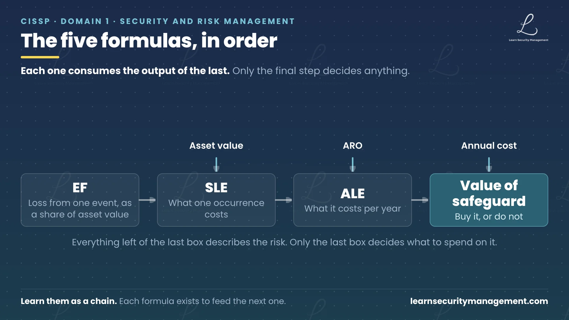
Each formula consumes the output of the one before it. Learning them in sequence is easier than learning them as five separate facts, because the chain explains why each exists.
Exposure factor and single loss expectancy
Exposure Factor (EF) is the proportion of an asset’s value that a single occurrence of the threat would destroy, expressed as a percentage or a decimal. A fire that would consume an entire warehouse has an exposure factor of 1.0. A breach that would compromise seventy percent of a database’s value has an exposure factor of 0.7.
EF  = monetary loss from one occurrence / asset value
SLE = asset value (AV) x EF
Single Loss Expectancy (SLE) is what one occurrence costs, in money. It is the asset’s value multiplied by the exposure factor.
The soft spot in both is asset value. It is the input everything downstream inherits, and it is rarely a number sitting in a system waiting to be read. Establishing it depends on someone knowing what the asset is, what it is worth to the business and what it would cost to replace, which is why asset valuation is a responsibility of the data owner rather than of the person running the calculation.
Annualized rate of occurrence and annualized loss expectancy
Annualized Rate of Occurrence (ARO) is how often the event is expected in a year. It is a frequency, not a probability, and it can exceed one. An event expected four times a year has an annualized rate of occurrence of 4. An event expected once every five years has an annualized rate of occurrence of 0.2.
ARO = number of occurrences / observation period in years
ALE = SLE x ARO
Annualized Loss Expectancy (ALE) is the expected cost per year. Annualising is the step that makes the whole method useful, because budgets are annual. A figure of 14,000 per year can be set beside a control costing 4,000 per year and the comparison is immediate.
The cost-benefit test that decides the purchase
The final formula is the only one that produces a decision rather than a description.
Value of safeguard = (ALE before - ALE after) - annual cost of safeguard (ACS)A positive result means the control returns more than it costs. A negative result means the safeguard costs more than the loss it removes, which makes it a poor purchase regardless of how well it addresses the threat. This is the punchline of the whole method, and it is the point most often lost: the goal is not the smallest possible risk, it is the best possible use of the next unit of budget.
A worked example, from asset value to funding decision
A server holding customer data is valued at 100,000. A breach would destroy seventy percent of that value. The organisation assesses the chance of such a breach at twenty percent in any given year.
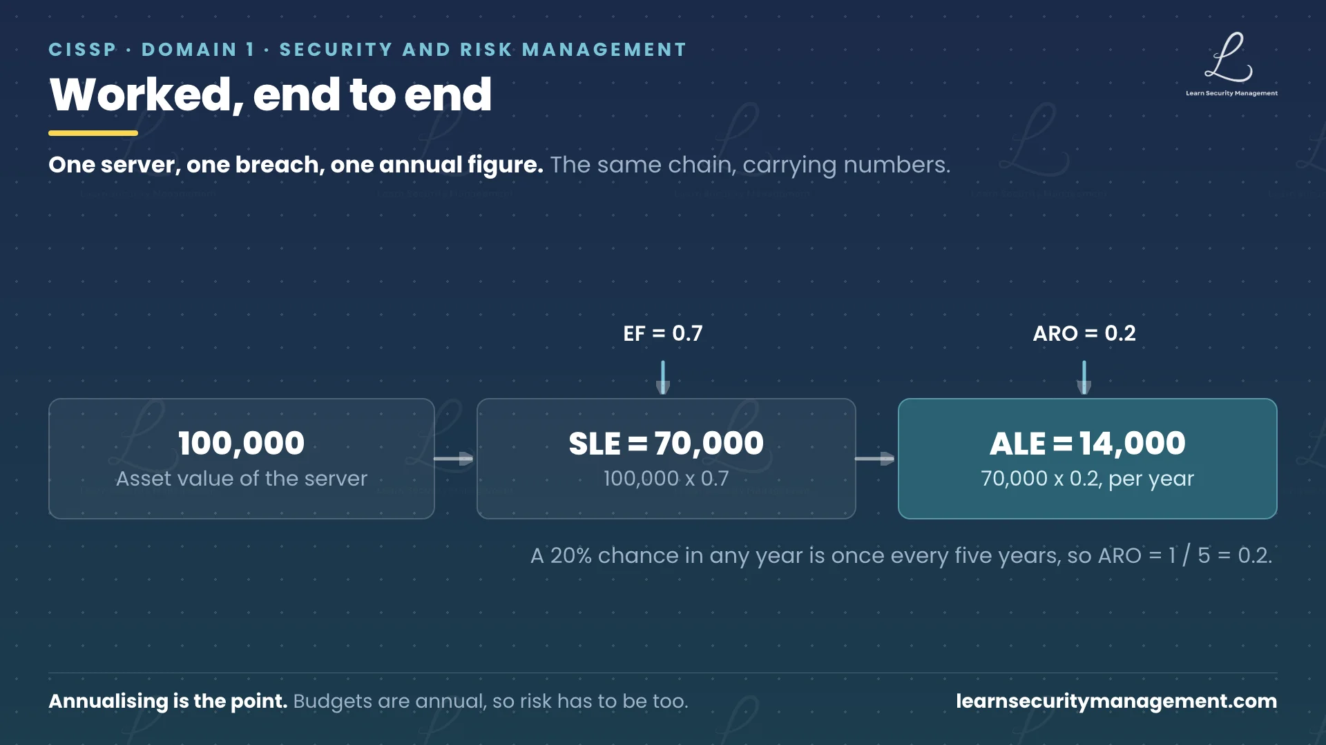
The exposure factor is 0.7, so the single loss expectancy is 100,000 multiplied by 0.7, which is 70,000. A twenty percent annual chance is the same as once every five years, so the annualized rate of occurrence is 1 divided by 5, which is 0.2. The annualized loss expectancy is therefore 70,000 multiplied by 0.2, which is 14,000 per year.
Now introduce a control. A safeguard is proposed that would halve the frequency of the event, taking the annualized rate of occurrence from 0.2 to 0.1. The new annualized loss expectancy is 70,000 multiplied by 0.1, which is 7,000 per year. The safeguard costs 4,000 per year to run.
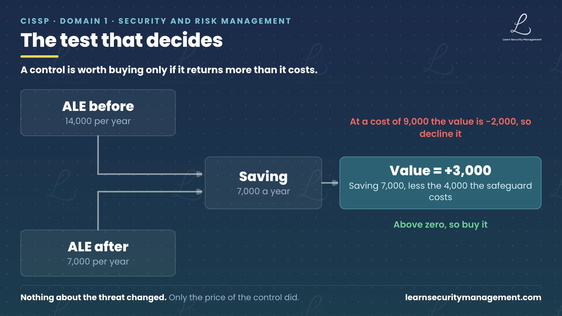
The annual saving is 14,000 minus 7,000, which is 7,000. Subtract the 4,000 the safeguard costs and the value of the safeguard is positive 3,000 per year. The control is worth buying.
Change one input and the answer inverts. If the same safeguard cost 9,000 per year, the calculation would be 7,000 minus 9,000, a value of negative 2,000, and the correct recommendation would be to decline it and consider a different treatment. Nothing about the threat changed; only the price did. That sensitivity is the reason the method is worth running rather than estimating.
Risk appetite, tolerance, limit and capacity
Numbers only help once an organisation has decided how much risk it is prepared to carry. Four terms bound that, and they are routinely used interchangeably in conversation when they mean different things.
| Term | What it bounds | Scope |
|---|---|---|
| Risk appetite | The total risk the organisation is willing to carry, setting the overall threshold | Aggregate, organisation-wide |
| Risk tolerance | The risk accepted for one specific asset and threat pairing | A single pairing |
| Risk limit | A quantitative maximum which, once crossed, triggers further action | A defined boundary |
| Risk capacity | The largest loss the organisation could absorb before its survival is in question | Absolute, organisation-wide |
The distinction that resolves most confusion is the first two: risk appetite is aggregate and organisation-wide, while tolerance applies to one asset and threat pairing. An organisation can hold a conservative appetite overall and still tolerate significant risk on a system it has judged non-critical.
Capacity is the one most often skipped, and it is the one that matters in a crisis. Appetite is a statement of preference and can be revised; capacity is a fact about the balance sheet. A programme whose accepted risks in aggregate approach its capacity has a governance problem no individual control will fix.
Inherent risk, residual risk and the controls gap
Inherent risk is the exposure that exists before anything is done about it. Applying controls closes part of the distance, the controls gap, and what is left afterwards is residual risk.
residual risk = total risk - controls gap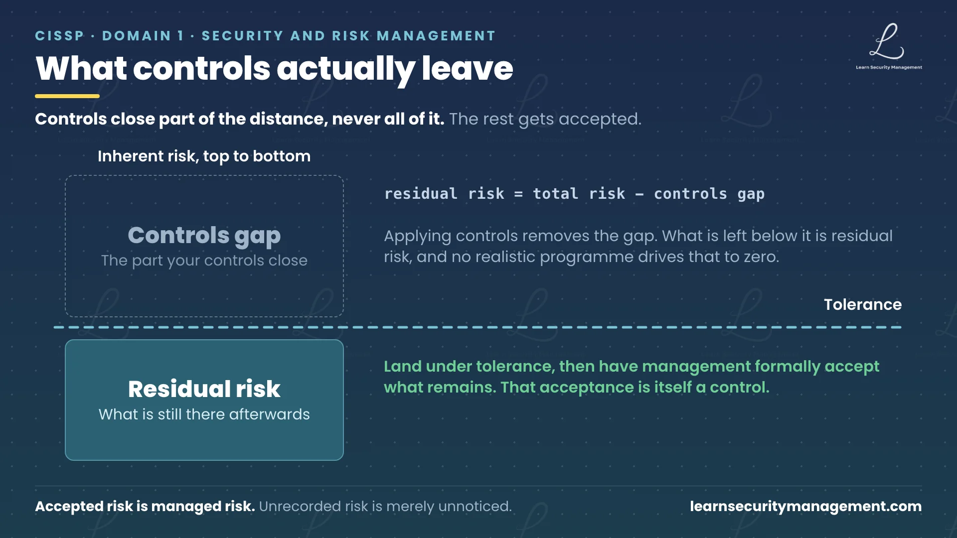
No realistic programme drives residual risk to zero, and treating zero as the target produces bad decisions in both directions: overspending on the last increment, and quiet dishonesty about what remains. The goal is to bring residual risk within the stated tolerance, at which point management formally accepts it.
That formal acceptance is a control in its own right. An accepted risk that has been documented, priced and signed off is being managed. The same risk left unrecorded is simply unnoticed, and the difference between the two becomes very visible after an incident. Acceptance is one of the four options in risk treatment, alongside mitigation, transfer and avoidance, and it is the only one that requires nothing to be built.
Where quantitative analysis breaks down
The formulas are arithmetic and will not fail. The inputs and the interpretation will.
The numbers inherit the quality of the estimates. Asset value and annualized rate of occurrence are frequently estimates presented with the confidence of measurements. A result carried to the nearest pound from inputs rounded to the nearest fifty thousand is precision theatre. Where an input is an estimate, the output should be reported as a range.
A negative cost-benefit result is an answer, not a failure. It says this particular safeguard is not the right response, and it should redirect attention to a cheaper control, a different treatment, or formal acceptance. Buying it anyway, because the risk feels alarming, is exactly the decision the method exists to prevent.
Low-frequency, high-impact events are poorly served. Annualising an event expected once in two hundred years produces a small annual figure that understates what happens when it occurs. Business continuity work exists partly because annualized loss expectancy is the wrong lens for a catastrophe, which is why a business impact analysis asks about maximum tolerable downtime rather than average annual cost.
Qualitative scores get read as precise. Low, medium and high are triage instruments. Once a heat map is built from them, the colours acquire an authority the underlying judgements never had.
Conclusion
The five formulas are worth knowing in sequence rather than individually, because the sequence is the argument: an asset has a value, an incident destroys a proportion of it, that happens at some frequency, and the annual figure that results is the only form in which risk can be compared with the cost of doing something about it. The cost-benefit test at the end is where the analysis stops describing and starts deciding.
The managerial habit underneath is more durable than the arithmetic. A risk stated as an annual figure, with a safeguard shown to return more than it costs, wins a budget conversation that technical alarm will lose. And once controls are in place, the residual risk that remains belongs to management as a documented, accepted decision against a stated tolerance. Pretending it has gone is not diligence.
Working these calculations under time pressure, with the numbers deliberately arranged to reward a careless read, is a different skill from following them on a page. The LSM CISSP practice questions include scenario items that turn on exactly these distinctions, including the annualized rate of occurrence expressed as a period rather than a rate, and the appetite-versus-tolerance trap.
Quick reference for the CISSP exam
The five formulas
- Exposure Factor (EF) = loss from one occurrence / asset value
- Single Loss Expectancy (SLE) = asset value x EF
- Annualized Rate of Occurrence (ARO) = occurrences / observation years
- Annualized Loss Expectancy (ALE) = SLE x ARO
- Value of safeguard = (ALE before minus ALE after) minus annual cost of safeguard
Conversions worth doing automatically
- Once every 5 years, ARO = 0.2. Once every 10 years, ARO = 0.1. Four times a year, ARO = 4.
- A percentage chance per year converts directly: 20% per year is an ARO of 0.2.
- Exposure factor is a proportion, so 70% is 0.7 and total destruction is 1.0.
The boundaries
- Risk appetite: aggregate, organisation-wide, sets the threshold.
- Risk tolerance: one asset and threat pairing.
- Risk limit: a quantitative maximum that triggers action when crossed.
- Risk capacity: the most the organisation could absorb and survive.
Common traps
- Reading appetite as tolerance, or quoting one figure as if it were the other.
- Treating a negative cost-benefit result as a reason to look for a better justification rather than a different control.
- Expecting residual risk to reach zero, instead of reaching tolerance and being formally accepted.
- Assuming a fully quantitative programme is the norm. Semi-quantitative hybrids are the realistic case.
- Confusing ARO as a frequency with probability. A frequency can exceed 1.